Popular ML algorithms
For the purposes of our workbench, we should not aim for a fine-grained repository of ML algorithm
classes. Of the hundreds of
distinct machine learning algorithms out there--thousands if we count variants and combinations; we should focus on categories that are recognizable by the
average practitioner. A practical consideration is also the manual labor involved in documenting each one of the classes which, in our case, means entering values for the selection criteria described in \ref{subsec:characterizing-algorithms}. Accordingly, the number of categories of algorithms should be comparable to that found in a typical cheat sheet.
While most authors would agree on the high-level breakdown of ML algorithms--typically by learning style--other divisions are possible, with further splits possible along many dimensions, including the nature of the inference task to be supported (e.g. classification vs. regression, vs. prediction), or the form of the trained model (e.g. decision tree vs. neural network), and its complexity (e.g. shallow vs. deep neural network).
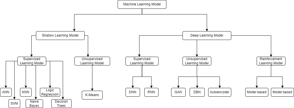
Given the current popularity of the deep learning family of algorithms, we built our ML taxonomy starting with the "deep" versus "shallow" dichotomy. Figure \ref{fig:ML-algorithm-taxonomy} shows such a taxonomy, edited from . Here, "deep" refers to neural networks with a large number of processing layers, while "shallow" covers a diversified set of approaches, including neural networks with few or undifferentiated layers. The next level of the taxonomy considers the
learning style, where we distinguished between supervised, unsupervised learning, and reinforcement learning. We enumerate the categories of algorithms below, and comment some of the choices.
The following list corresponds to a depth-first traversal of the hierarchy of Figure \ref{fig:ML-algorithm-taxonomy}, starting from the top (supervised vs. shallow):
- ANN: Artificial Neural Network . It refers to the first generations of neural networks (e.g. multi-layer perceptron), and may be called "shallow ANNs" in contrast to the more recent and efficient 'deep learning models'.
- SVM: Support Vector Machine . SVM outperformed ANN in many tasks before the advent of deep learning networks. It is still an approach of choice for binary classification and anomaly detection given its parameter frugality and its grounding on statistical optimization.
- KNN: K Nearest Neighbor . This simple classification algorithm is easy to implement and requires no training before use. It is very efficient for small sets, but does not scale well with bigger data or dimensions. It is also sensitive to noise.
- Naive Bayes . This powerful probabilistic classification technique relies on matching hypotheses against the supporting evidence. It is simple to implement, fast, and can learn from relatively small data sets, but relies on well-behaved data (independent predictor variables).
- Logistic regression : This approach matches numerical data against a straight line, before applying a logistic function for binary classification. It is simple to implement and inherently explainable, but it too relies on the linearity and independence of the input variables.
- Decision trees. Their use of if-then-else rules makes them easily explainable. They are easy to implement, but are computationally complex for large attribute sets, becoming prone to overfitting and losing their readability. Finding minimal trees, under quality constraints, is also a challenge.
- K-Means: . This technique is somewhat related to K-NN, but the number of classes is determined beforehand, and the class centroids are sensitive to initial values. It is easy to implement, but the efficiency training depends on the number of classes (k), the homogeneity of class distributions, and the absence of outliers.
And now with the
deep learning models, starting with models for supervised learning (Figure \ref{fig:ML-algorithm-taxonomy}). They are currently the most accurate neural models when sufficient labeled data are available for training:
- DNN (Deep Neural Network) : This architecture is commonly used for classification and prediction. Two popular models are convolutional neural networks (CNNs) and Transformers . Both models rely on stacked feature extraction and by shallow ANNs . The the two models differe by the nature of the features and the way they are obtained.
- RNN (Recurrent Neural networks) : RNN uses feedback as a processing context. It is well suited for processing sequences such as textual information and time series. Popular variants replace the neuron elements by LSTM (Long Short-Term Memory) or GRU (Gated Recurrent Units) cells for improved efficiency. Bidirectional RNNs (Bi-RNNs) use two RNNs running in opposite directions for even better contexts.
The models with unsupervised learning can be divided as follows:
- GAN (Generative Adversarial Network) . This model focuses on learning the distribution of the training data in order to generate similar data. It is used in applications such as object transformation, sequence translation, and even artistic creation in the style it was trained on. It is also used in less benign ones such as fake news and fraud.
- DBN: Deep Belief Networks can be viewed as the precursors of today's deep learning architectures, since they aim at a hierarchical representation of the input data. They perform unsupervised learning with unlabeled data, eventually followed by fine-tuning with labeled input; today's popular ChatGPT DNN model is based on the same principles. Their complex architecture requires substantial computational resources.
- Autoencoder : This model aims to learn an efficient coding of unlabeled data, by projecting the input onto an intermediate space and then reconstructing the input from this representation. Autoencoders may, in some cases, project the data into a higher-dimensional space before pruning the elements with regularization functions (e.g. ). They can be used for noise filtering (e.g. ), and turned into generative models (e.g. ).
The last category in the list,
reinforcement learning (RL) algorithms, is useful for building decision-making systems. Here, the purpose is to evaluate the merit of different actions to reach a desired outcome. We distinguish between two flavors, one that models the actions within a set environment and the other that just aims the maximize their cumulative value (reward).
- Model-based RL: This approach typically follows Markov decision process (MDP), whith actions causing probabilistic state transitions, and reaping rewards associated with the target states. It is capable of fast decisions, but suffers from the limitations of Markov processes, including poor scalability. Still, it has been used with great success in robotics and to build game algorithms that defeat human champions (e.g. AlphaGo)
- Model-free RL: This model simply seeks to maximize a cumulative reward function that includes future actions, using an iterative procedure that trains a DNN to learn the optimal policy. Model-free RL models are typically slow learners. Two popular ones are Q-learning and temporal differences .
Notice that we did not include in our taxonomy ensemble learning techniques and various ML meta-heuristics (bagging, gradient boosting, etc.) that have been developed to remedy weaknesses in existing algorithm families (overfitting, sensitivity to noise, etc.) or problems with datasets (unbalanced, noisy, etc.); those are 'orthogonal' to the taxonomy of Figure \ref{fig:ML-algorithm-taxonomy}, and can be applied in conjunction with many of the algorithm families shown in Figure \ref{fig:ML-algorithm-taxonomy}.
Neither did we include hybrid models that combine learning modalities.